Marine use case

Summary:
Discussions with the team at the Integrated Marine Observing System (IMOS) revealed a treasure trove of Marine data in the Australian Ocean Data Network (AODN) Portal that had not yet been explored using the analytical tools available at EcoCommons. Here we demonstrate how these marine data predict migration patterns of two marine species, the Yellowtail Kingfish (Seriola lalandi) and the Bull Shark (Carcharhinus leucas). The R code used to generate these results is provided and could be run on the Ecocommons’ coding cloud after 29 November.
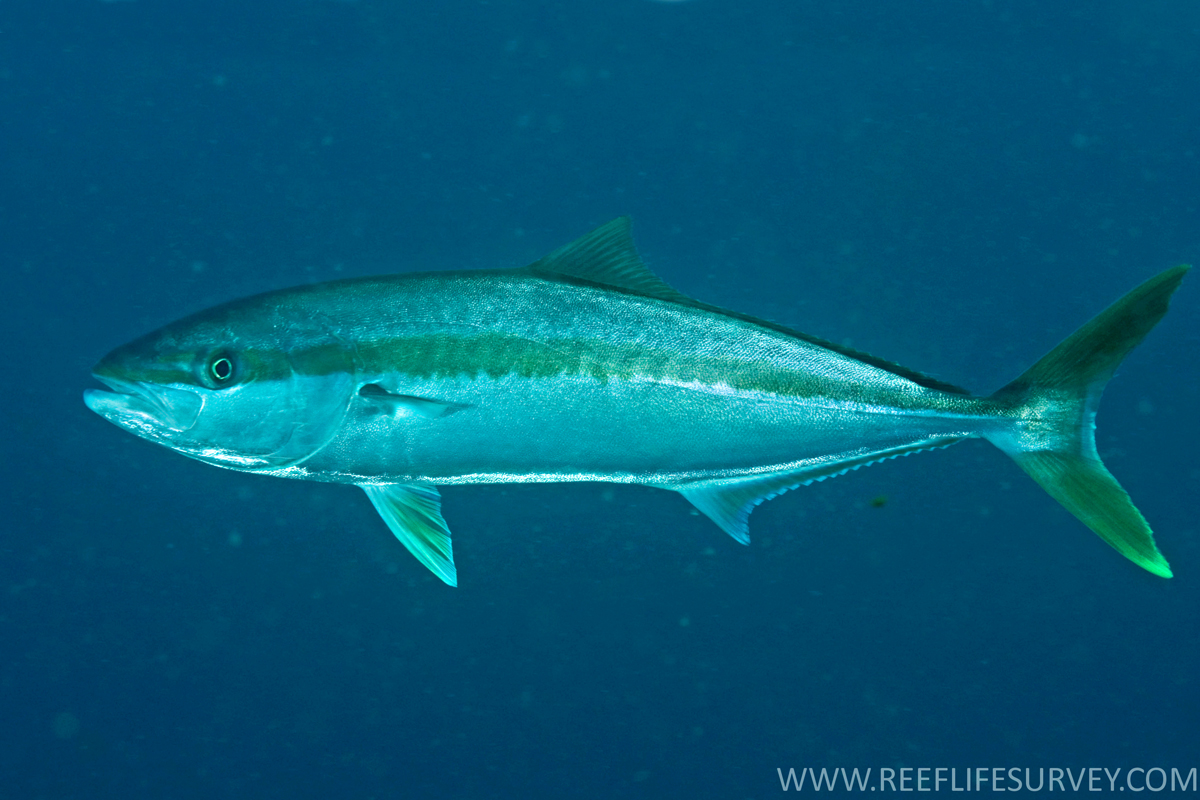
By – Rick Stuart Smith
Figure 1. This is a prediction of Yellowtail Kingfish distribution for each month. The results are averaged from 2011 to 2021 and are repeated multiple times to show the predicted changes during migration.
Introduction:
IMOS includes 13 facilities that monitor marine environments. The resulting systematic long-term data are then made available through the AODN. These data include a variety of large-scale datasets on marine conditions as well as growing volumes of occurrence data from tracked marine species. Marine species with tags are tracked with a network of acoustic sensors deployed widely in Australian near-shore marine environments. Together the team at EcoCommons recognised that these data could be used to generate predictions of species distributions using existing workflows. As the teams worked together, it became clear that there was good spatial and temporal data available. We, therefore, sought to capture the seasonal movements of marine species using these rich data.
EcoCommons has a few point-and-click dashboards which include the capacity to model species distributions at different time periods. This migratory modelling workflow generates a separate model for each season or month. This is a useful workflow when very different environmental variables are important to species in different seasons and when the sampling of species occurrences between seasons is roughly equivalent. Here we opted to demonstrate how a workflow coded in R could pull data from each month to generate one model that then could be used to predict a distribution for each month of the year.
Here we sought to demonstrate how some of the vast marine data available through AODN could be used within EcoCommons’ R environment to capture migratory movements of marine species.

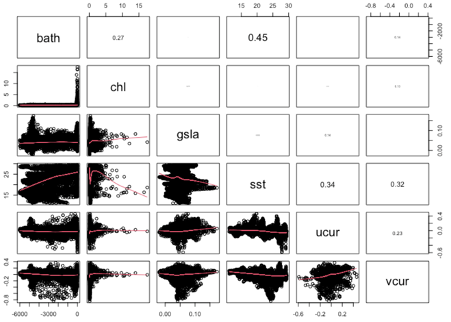
Figure 2. Pairwise correlation between environmental rasters based on 1000 random locations within the study area.
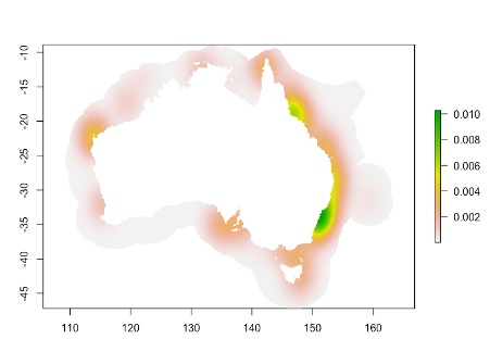
Figure 3. Map based on kernel density based on the total number of days a sensor was deployed at each location. Background points are then selected with the probability of selection based on these values, with areas with higher values more likely to be selected. This allows the background points to be selected from areas with the same spatial bias as present in the sensor deployments.
Methods:
Occurrence data for both the Yellowtail Kingfish and Bull Shark came from the IMOS Animal Tracking Facility. The model for Yellowtail Kingfish was based on over 22,000 records, while the Bull Shark model was based on over 24,000 records. Both sets of data were filtered for spatial and temporal duplicates at monthly time periods within ~925m square grid cells. As both of these were presence data only datasets, we opted to use the machine learning algorithm Maxent.
Environmental variables included the marine variables:
- Chlorophyll – A
- Gridded Sea Level Anomaly
- Sea Surface Temperature
- And north – south current velocity (VCUR)
All data was run through quality assurance and quality control processes following (Hoenner et al. 2018). The source data used here are available through the R package remora.
Month (i.e. 12, 11, 10, …) was also used as a factor, and bathymetry and distance to coast were trialled in initial models but later dropped.
Bathymetry data had the resolution and rough extent that we wanted to use for all environmental variables. Some acoustic sensors were deployed in bays or shallow water too close to shore to be overlapped by bathymetry or other marine environmental grids. In order to estimate values, where these nearshore sensors were deployed, average values were generated based on the close cell values to extend the boundary of the grid to the shore using the raster R package with the focal function (see line 65 of the R script).
For each environmental variable where there were years of monthly data or there were daily data available an average value was calculated for each month. This resulted in twelve folders, one for each month, with a set of the same monthly averaged variables, where each variable in each folder had the same name, one that also matched the name used for each column of data used to generate the model. Each of these variables was processed in a loop (see line 145 of the R script) where each raster with the same month in the file name was read in, stacked, averaged, and adjusted to the same resolution as the bathymetry data with the raster function ‘projectRaster’. The focal function was then used to fill in missing values close to the shore; the boundary was then set to match the bathymetry data and the averaged raster was written to the appropriate month file. Correlations between grids were checked with a correlation matrix (Figure 2) based on 1000 random point locations (see R script: lines 302 – 314). Highly correlated variables would have been removed.
Figure 4. This is a prediction of Bull Shark distribution for each month. The results are averaged from 2011 to 2021 and are repeated multiple times to simply show the predicted changes during migration.
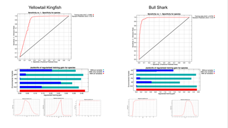
Figure 5. ROC curve provides an assessment of sensitivity and specificity of model predictions with a Yellowtail Kingfish AUC = 0.880 and Bull Shark AUC = 0.979. Response curves indicate how the probability of occurrence varies as each environmental variable increases on the x-axis. Jackknife variable importance plots suggest that Sea Surface Temperature (sst), and Cholophyll (chl) were the most important variables in both models, with east-west surface current velocity (vcur) important for Yellowtail Kingfish.
Maxent uses a default of 10,000 randomly generated points instead of absence data, but work has shown that drawing data from a bias layer is one way to improve results. There are a variety of ways to generate a layer that captures uneven sampling effort. In this case, detections were only possible in areas where acoustic sensors had been deployed, so we simply took the sum of days when monitors were deployed in any grid cell. We then used the MASS package function kde2d to generate a two-dimensional kernal density estimation (Figure 3) based on the occurrence point locations (line 112 of the R script). We added the coordinates from the bounding box to the occurrence point locations to match the extent of the whole study area (lines 201 – 205). There are a variety of other approaches which would also generate similar results.
Occurrence locations were then turned into a spatial points layer (line 49). A loop was then constructed to run through each folder of monthly data and extract the environmental values for each occurrence point that was collected during that same month (R script, lines 103 – 105). Within each month we also generated 2000 points sampled from the bias file (line 366). The 12 resulting data-frames were appended together and the variable month was set as a factor. This data-frame included all the occurrence locations, and all the locations selected as background points based on the bias file. A vector that indicated which row was either a presence ‘1’ or background ‘0’ was also set.
The single maxent model based on all these monthly data was run using the dismo package with the maxent function (line 400). This model included arguments (line 398) that removed duplicate cells, included jackknife variable importance, response curves and plots. Importantly, after initial runs we decided to adjust the regularization so we increase the beta-multiplier to 3 to ensure predictions had a more spread-out distribution. Initial models also indicated that bathymetry and distance to the coast variables led to predictions that were too narrowly tied to the coast. For these reasons, these variables were dropped in the final model.
The final step we undertook in this demonstration model was to use this model to make a prediction into each month (R script, lines 409 – 449). Again, in order for this to work in this framework is to ensure each month has a separate file for each variable used in the model, and those variable names need to match the column names given for the variables in the data-frame used to run the model.
Results:
The available marine data were sufficient to identify broad patterns of seasonal distribution changes associated with migration (Figures 1 & 4) which expert review indicated were reasonable estimates. AUC reported in this model indicated the Yellowtail Kingfish model predicted training data relatively well with AUC = 0.880 while Bull Shark model reported a very high AUC of 0.979 (Figure 5). During initial modelling iterations for Yellowtail Kingfish, AUC varied between runs and was sensitive to slight changes in model arguments or environmental variables. We suspect AUC scores for the Bull Shark might also vary with multiple runs, but only ran this model once. Further, both species had predicted distributions in some areas where the species are not believed to occur. This suggests that while the habitat might seem suitable based on the variables included, other variables which might be important for the distribution of these species were not included in this model. A series of absence data from areas and times where sensors did not detect these species may also improve these models. Nonetheless, these initial results do pick up the broad patterns of migratory distributions and variable response curves and importance plots appeared reasonable (Figure 5).
Discussion:
IMOS and the data available through AODN open the door to many analyses of the Austral marine environment. Species distribution modelling has been long recognised as an important tool for species conservation, as knowing where species occur is the first step in conserving or managing populations. In the last decade, a growing number of studies have explored species distributions during migrations and here we supply a framework to develop models that can capture the distributions of species that vary over time. Many marine species range widely, and while tracking studies are increasing our understanding of the movements of marine species, this framework provides a method to explore likely patterns of movement for a growing number of species. Understanding temporally-dynamic distributions are important when setting fisheries targets and regulations, or planning spatial management that need to provide protection throughout species migratory journeys. Further, it is likely that climate change will impact migratory species, and these kinds of models could be used as the foundation to predict likely future migration patterns expected under climate change.
At EcoCommons we are fond of saying that all models are wrong, but some are useful. These models appear to be capturing broad seasonal movement patterns of species, but there are a variety of ways these models could be improved including through using additional tools available at EcoCommons. For example, here we selected a presence only method, Maxent, to predict distributions, but if we inferred zeros at monitoring sensors in months where other species were detected but our target species was not observed, many other machine learning and statistical models could be used. It is likely that the inclusion of zeros in a model would reduce the over predictions into areas where the species is not thought to occur. Alternatively, the study area could be restricted to only include those areas where the species is likely to occur. As with any SDM, these models would also be improved with higher resolution data, more comprehensive sampling-based occurrence data, and with environmental predictors known to be ecologically critical for each species. Finally, these models should be viewed as preliminary until they are validated more fully. This could be done with 25% of the data set aside before training the model to be used for testing, or better by an independent dataset. (see step 4 – for validation of predictions using independent data on static SDMs)
Finally, there are a huge variety of modelling frameworks in both marine and terrestrial ecology, and it is hoped that an increasing volume of those workflows will be made publicly available on EcoCommons. Please get in touch if you have some useful code you would like to share in our growing code library.
Our partners





- EcoCommons Australia partners with the Australian Research Data Commons (ARDC), which is supported by funding from the National Collaborative Research Infrastructure Strategy (NCRIS) https://doi.org/10.47486/PL108.

